For all that I like using Blender as a tool to visualize molecular structures, there are obvious tradeoffs when using general-purpose software instead of something customized for chemistry. One of those tradeoffs is that there’s no obvious way to import various kinds of computational chemistry data.

For me, this is most often molecular orbitals, which we occasionally want to show in manuscripts. So, I started to think a bit about how to render isosurfaces in combination with imported geometries. I briefly considered trying to write something that processes cube files (from Gaussian), but quickly gave up. Instead, I’ve found that Jmol does the job wonderfully, and with minimal fuss.

Here’s the process, step-by-step, assuming you’re starting with a Gaussian cube file. I’m not a very sophisticated Jmol user, and I’m sure I’m missing out on a lot of its power, but this works as a way to just get the geometry in Blender. If you want to try this out and don’t have a cube file handy, feel free to download the one I used.

1. Open Jmol and start the console (File/Console).
2. Load the geometry:

   load /path/to/file/file.cub

3. Write the pdb:

   write filename.pdb

   

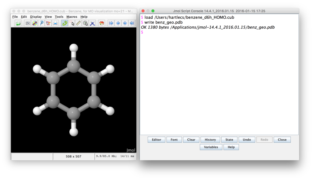
   Jmol screenshot. The Gaussian cube file has been loaded and the geometry written to a pdb file.

4. Clear the geometry:

   delete all

5. Generate the first isosurface and write the first wrl file. Cutoffs of 0.02 are reasonable for MOs. For the total density, 0.0004 works well.

   isosurface name1 cutoff +0.02 "/path/to/file/file.cub"
   write filename_a.wrl

   

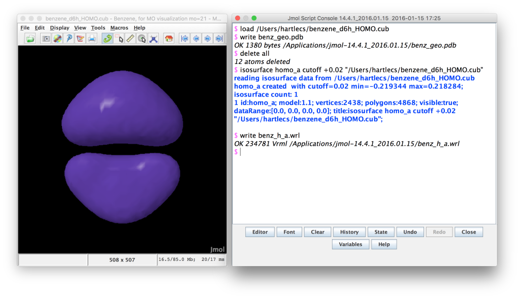
   Jmol screenshot. The positive lobes of the MO have been loaded and written to a wrl file.

6. For MOs, generate the second (negative) isosurface after removing the first one:

   isosurface name1 off
   isosurface name2 cutoff -0.02 "/path/to/file/file.cub"
   write filename_b.wrl

   

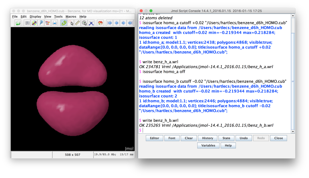
   Jmol screenshot. The negative lobes of the MO have been loaded and written to a wrl file.

7. Exit Jmol:

   exitJmol

At this point, you should have three files (filename.pdb, filename_a.wrl, and filename_b.wrl), probably sitting in your Jmol folder if, like me, you were too lazy to specify a specific path. These should now be ready for Blender.

1. Open Blender, and, assuming you use one, open a template with camera and lighting placement (my default setup is discussed/included in my blmol post).
2. Load the geometry as discussed in the blmol instructions, using the native Python interface. Note that the units must be changed to angstroms (from the default of nm). This gives a gigantic structure (which can be shrunk later), but is necessary to match up with the isosurface.

   import blmol
   M = blmol.Molecule()
   M.read_pdb("/path/to/file/filename.pdb")
   M.draw_bonds(units="A")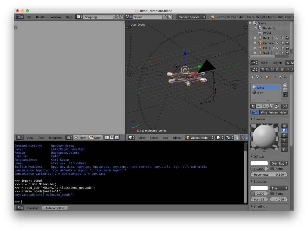

   

   Blender screenshot. The geometry has been loaded and drawn using the blmol script.

3. Import both wrl files (File/Import/X3D Extensible 3D). If the positive and negative lobes of an MO are loaded, I’d recommend joining them at this point (select both and hit ctrl-j).
   

   Blender screenshot. Both parts of the isosurface have been loaded, but are out of alignment with the geometry.

4. You will notice at this point that the geometry and the isosurface are out of alignment; however, this is easily corrected. Select the isosurface and rotate about the x-axis by −90°, then about the z-axis by 180° (“r x -90” and then “r z 180”). This appears to work for MOs, although I have had issues getting total densities aligned properly. It’s a good idea to reference against a visualization done in another program, if available (e.g., Gaussview).
   

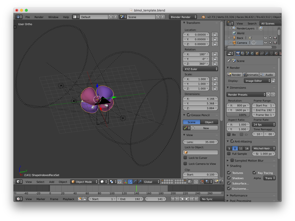
   Blender screenshot. The MO is now aligned with the geometry. The objects can now be scaled and positioned for rendering.

5. Probably a good idea to set the geometry as the parent of the isosurface (select the isosurface, then the geometry, then ctrl-p).
6. At this point I scale the model by a factor of 0.1 to switch the units to nm, reset the origin of the geometry to its center, and move it in front of my camera.

After shrinking and positioning the camera, here’s what I get:

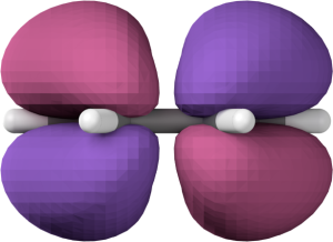
Blender rendering of one benzene HOMO, without any tweaking.

It’s ok, if perhaps not amazing, but the important point is that the MO is now loaded into Blender and ready to be tweaked. Here’s the same image after changing the materials, switching to smooth shading, and applying the smooth modifier.

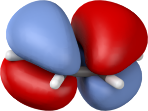
HOMO of benzene, rendered in Blender.

And here’s a similar image produced in GaussView:

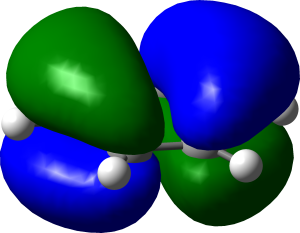
Benzene HOMO rendered in Gaussview.

While I wouldn’t claim there’s any scientific difference between the two, I like the softer reflections and shading in Blender.

Just for the heck of it, here’s an animation cycling through of benzene and its six π-orbitals. Setting up the animation was pretty easy (perhaps 10–15 minutes of work, not counting the time it took to remember how to do simple animation). Took almost 12 h to render, though, because I forgot to switch off raytraced shadows.